Invariant Calculation Example

In the following example, we demonstrate the calculation and plotting of invariant points with quantified uncertainty.

Set-up

First we import all of the required packages, and set the seaborn color codes so that we have pretty plots later.

import matplotlib.pyplot as plt
import numpy as np
import seaborn as sns
from dask.distributed import Client
from distributed.deploy.local import LocalCluster
from pycalphad import Database, equilibrium, variables as v
from pduq.invariant_calc import invariant_samples
from pduq.uq_plot import plot_contour
sns.set(color_codes=True)

Now we use dask distributed to start up a cluster so we can do our invariant calculations in parallel. Set n_workers to the number of cores/processes on the cpu or fewer.

c = LocalCluster(n_workers=8, threads_per_worker=1)
client = Client(c)
print(client)

By printing the client we can see that we have the correct number of workers.

<Client: scheduler='tcp://127.0.0.1:56581' processes=8 cores=8>

Now we load the database file, and load the parameter sets into a numpy array with the following shape: (# parameter sets, # parameters)

dbf = Database('CU-MG_param_gen.tdb')
params = np.load('trace.npy')[:, -1, :]

Invariant Calculations

We then set up and run the invariant calculation for all of our parameter sets using the invariant_samples function from the invariant_calc module. We start by defining the important variables. This includes a guesses for the composition of the invariant and for the temperature bounds.

X = .2  # X_MG guess for invariant
P = 101324  # pressure
Tl = 600  # lower temperature bound for invariant
Tu = 1400  # upper temperature bound for invariant
comp = 'MG'  # species to reference for composition

Tv, phv, bndv = invariant_samples(
    dbf, params, X, P, Tl, Tu, comp, client=client)

Data Analysis and Plotting

Now that the calculation has completed, let’s calculate the mean composition and temperature of the invariant:

print('mean invariant composition:', np.mean(bndv[:, 1]))
print('mean invariant temperature:', np.mean(Tv))

mean invariant composition: 0.21396602343616997
mean invariant temperature: 1003.1419270833334

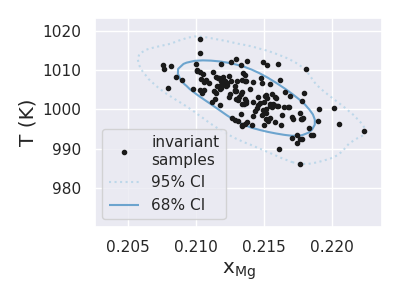
Let’s also plot the invariant points calculated for each parameter set and some uncertainty contours

# form an array for the invariant points
points = np.zeros((len(Tv), 2))
points[:, 0] = bndv[:, 1]
points[:, 1] = Tv
c = sns.color_palette("Blues", 2)

plt.figure(figsize=(4, 3))

# plot the raw invariant points
plt.plot(points[:, 0], points[:, 1], 'k.',
         label="invariant\nsamples")

# plot KDE estimated uncertainty intervals
plot_contour(points, c, 0.6)

plt.xlabel(r'$\mathrm{x_{Mg}}$', fontsize="large")
plt.ylabel('T (K)', fontsize="large")
plt.tight_layout()
plt.legend()
plt.show()

resulting in the following figure

Finally, we can calculate how many of the total 150 points fall within some desired composition and temperature domain

reg = (.212<=points[:, 0])*(points[:, 0]<.217)* \
      (999<=points[:, 1])*(points[:, 1]<1007)
print('points for .212<=X<.217, 999<=T<1007:', np.sum(reg))

points for .212<=X<.217, 999<=T<1007: 51

This means that the invariant has 34% probability of falling in the defined region