Single Point Equilibrium Calculation and Analysis

In the following example, we demonstrate the simultaneous calculation of single point phase equilibria for multiple Gibbs energy parameter sets in CALPHAD using PDUQ. We then perform typical analyses on the results.

Set-up

First, we import all of the required packages.

import numpy as np
from dask.distributed import Client
from distributed.deploy.local import LocalCluster
from pycalphad import Database, variables as v
from pduq.dbf_calc import eq_calc_samples
from pduq.uq_plot import get_phase_prob, plot_dist

Now we use dask distributed to start up a cluster so we can do our equilibrium calculations in parallel. Set n_workers to the number of cores/processes on the cpu or fewer.

c = LocalCluster(n_workers=8, threads_per_worker=1)
client = Client(c)
print(client)

By printing the client we can see that we have the correct number of workers.

<Client: scheduler='tcp://127.0.0.1:56581' processes=8 cores=8>

Now we load the database file, and load the parameter sets for the last 5 converged iterations of our ESPEI MCMC run into a numpy array with the following shape: (# parameter sets, # parameters) or (750, 15)

dbf = Database('CU-MG_param_gen.tdb')
params = np.load('trace.npy')[:, -5:, :].reshape((150*5, 15))

Equilibrium Calculations

We then set up and run the equilibrium calculations for our 750 parameter sets using the eq_calc_samples function from the dbf_calc module. We first define the equilibrium conditions for our single point, and then calculate the equilibria.

# Define the equilibrium conditions including pressure
# (Pa), temperature (K), and molar composition Mg
conds = {v.P: 101325, v.T: 1003, v.X('MG'): 0.214}

# perform the equilibrium calculation for all parameter
# sets
eq = eq_calc_samples(dbf, conds, params, client=client)

Data Analysis and Plotting

Now that the calculation has completed, let’s calculate the probabilities of each phase combination having a non-zero phase fraction:

# define a list of phase regions
phaseregLL = [['FCC_A1', 'LIQUID'], ['LIQUID'],
              ['LAVES_C15', 'LIQUID'],
              ['FCC_A1', 'LAVES_C15']]

# calculate the probability of non-zero phase fraction
for phaseregL in phaseregLL:
    prob = get_phase_prob(eq, phaseregL)
    print(phaseregL, ' ', np.squeeze(prob.values))

['FCC_A1', 'LIQUID']   0.21066666666666667
['LIQUID']   0.23333333333333334
['LAVES_C15', 'LIQUID']   0.04133333333333333
['FCC_A1', 'LAVES_C15']   0.5146666666666667

From this analysis we have discovered that there is a roughly 51% probability of the FCC_A1 + LAVES_C15 phases having a non-zero phase fraction.

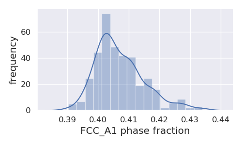
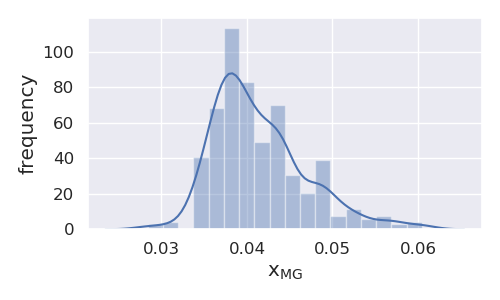
Let’s also plot distributions for the FCC_A1 phase fraction and composition when there is a non-zero FCC_A1 + LAVES_C15 phase fraction:

coordD = {'T':1003, 'X_MG':.214, 'component':'MG'}
phaseregL = ['FCC_A1', 'LAVES_C15']
phase = 'FCC_A1'

# plot the phase fraction
uq.plot_dist(eq, coordD, phaseregL, phase, typ='NP', figsize=(5, 3))

# plot the phase composition
uq.plot_dist(eq, coordD, phaseregL, phase, typ='X', figsize=(5, 3))

resulting in the following figures