Phase Diagram Calculation and Analysis

In the following example, we demonstrate the simultaneous calculation of phase diagrams for multiple Gibbs energy parameter sets in CALPHAD using PDUQ. We then produce a variety of phase diagram representations with uncertainty.

Set-up

First, we import all of the required packages.

import numpy as np
import seaborn as sns
from dask.distributed import Client
from distributed.deploy.local import LocalCluster
from pycalphad import Database, variables as v
from pduq.dbf_calc import eq_calc_samples
from pduq.uq_plot import plot_phasereg_prob, plot_superimposed

Now we use dask distributed to start up a cluster so we can do our phase diagram calculations in parallel. Set n_workers to the number of cores/processes on the cpu or fewer.

c = LocalCluster(n_workers=8, threads_per_worker=1)
client = Client(c)
print(client)

By printing the client we can see that we have the correct number of workers.

<Client: scheduler='tcp://127.0.0.1:56581' processes=8 cores=8>

Now we load the database file, and load the parameter sets for the last iteration of our ESPEI MCMC run into a numpy array with the following shape: (# parameter sets, # parameters) or (150, 15)

dbf = Database('CU-MG_param_gen.tdb')
params = np.load('trace.npy')[:, -1, :]

Equilibrium Calculations

We then set up and run the equilibrium calculations for our 150 parameter sets using the eq_calc_samples function from the dbf_calc module. We first define the equilibrium conditions for our single point, and then calculate the equilibria. Using the current version of pycalphad, calculating all 150 phase diagrams will take several hours on a desktop computer. This will be significantly faster in upcoming releases. You can check the progress in the pduq.log file that is automatically generated.

# equlibrium conditions including the pressure (Pa),
# temperature evaluation points (K), and molar
# composition MG evaluation points
conds = {v.P: 101325, v.T: (300, 1500, 10), v.X('MG'): (0, 1, 0.01)}

# perform the equilibrium calculation
eq = eq_calc_samples(dbf, conds, params, client=client)

Phase Diagram Uncertainty Visualization

Let us first visualize the uncertainty in the phase boundaries by superimposing the phase diagrams with uncertainty.

# We can assign colors to the phase names so
# that they are the same in all of the plots
phaseL = list(np.unique(eq.get('Phase').values))
if '' in phaseL: phaseL.remove('')
nph = len(phaseL)
colorL = sns.color_palette("cubehelix", nph+2)
cdict = {}
for ii in range(nph):
    cdict[phaseL[ii]] = colorL[ii]

# we can also specify a dictionary to have pretty
# labels (even LaTeX) in our plots
phase_label_dict = {
    'LIQUID':'liquid', 'FCC_A1':'FCC', 'HCP_A3':'HCP',
    'CUMG2':r'$\mathrm{Cu{Mg}_2}$', 'LAVES_C15':'Laves'}

# plot the superimposed phase diagrams
uq.plot_superimposed(eq, 'MG', alpha=0.2,
                  xlims=[-.005, 1.005], cdict=cdict,
                  phase_label_dict=phase_label_dict,
                  figsize=(5, 4))

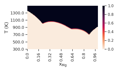
Now we plot the probability of non-zero phase fraction for the liquid phase over all 150 Gibbs energy parameter sets versus composition and temperature.

uq.plot_phasereg_prob(
    eq, ['LIQUID'], coordplt=['X_MG', 'T'], figsize=(5, 3))