Uncertainty Quantification for Thermodynamic Properties
In the following example, we leverage the multiple parameter sets resulting from ESPEI to plot thermodynamic properties (Cp, H, S, and G) with quantified uncertainty.
Set-up
First, we import the plot_property function from the uq_plot module.
from pduq.uq_plot import plot_property
Now we load the database file, and load the parameter sets for the last converged iterations of our ESPEI MCMC run into a numpy array with the following shape: (# parameter sets, # parameters) or (150, 15)
dbf = Database('CU-MG_param_gen.tdb')
params = np.load('trace.npy')[:, -1:, :]
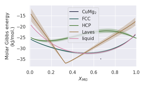
Plotting Molar Gibbs Energy
Let’s go ahead and plot the molar Gibbs energy versus molar composition at a fixed temperature.
comps = ['MG', 'CU', 'VA']  # species to consider
T = 650  # temperature in Kelvin
prop = 'GM'  # property of interest (molar Gibbs energy)
ylabel = 'Molar Gibbs energy\n(kJ/mol.K)'  # y-axis label
yscale = 1e-3  # we want to scale the Gibbs energy to give kJ/mol.

# we can now plot the property. Note that phaseL, phase_label_dict,
# and cdict are defined in the phase diagram prediction example
uq.plot_property(dbf, comps, phaseL, params, T, prop,
                 phase_label_dict=phase_label_dict,
                 ylabel=ylabel, yscale=yscale, cdict=cdict,
                 xlim=[-0.005, 1.005], figsize=(5, 3))
PDUQ will provide the following output during plotting,
starting GM evaluations for the CUMG2 phase
phase is a line compound
starting GM evaluations for the FCC_A1 phase
starting GM evaluations for the HCP_A3 phase
starting GM evaluations for the LAVES_C15 phase
starting GM evaluations for the LIQUID phase
telling us when the evaluation of the energies of each phase has begin and that the CUMG2 phase is being treated as a line compound.
Finally, PDUQ will produce the following figure.
Plotting Molar Enthalpy of Mixing
Let’s go ahead and plot the molar enthalpy of mixing versus molar composition at a fixed temperature.
T = 298.15  # temperature in Kelvin
prop = 'HM_MIX'  # property of interest (molar enthalpy of mixing
ylabel = 'Molar Gibbs energy\n(kJ/mol.)'  # y-axis label
yscale = 1e-3  # we want to scale the Gibbs energy to give kJ/mol.

# we can now plot the property. Note that phaseL, phase_label_dict,
# and cdict are defined in the phase diagram prediction example
uq.plot_property(dbf, comps, phaseL, params, T, prop,
                 phase_label_dict=phase_label_dict,
                 ylabel=ylabel, yscale=yscale, cdict=cdict,
                 xlim=[-0.005, 1.005], figsize=(5, 3))
Producing the following figure. Note that the CuMg2 energy is hidden beneath the Laves energy.
